Activity 19: Probabilistic Classification

Probabilistic classification via LDA (Linear Discriminant Analysis) is performed on the compiled data of the training set images (from Activity 18). It is done by assuming the distribution and then obtaining the probability theoretically. Assuming that each class (considering each kind of food constitutes a class) has multivariate normal distribution and all in the group have the same covariance matrix, we get what is called the LDA formula:

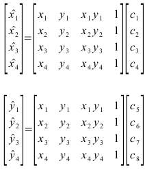
A number was assigned to each object, then from the equation object k was assigned to group i that has the maximum f_i.

The process was then repeated on the test set images to investigate whether it classifies the object under their correct class.

From the last activity, I've chosen the kwek-kwek and pillows to be the two different classes, mostly because they are the easiest to identify by observation alone, just to simplify the automatic process. The chosen features to act as predictor variables are the same features chosen in activity 18.

The training set:

Obtained f1 and f2 values.
f1 f2
9420.1989 9419.4684
9752.2214 9751.3123
9731.9091 9731.8893
9710.5355 9709.5048
9679.0613 9679.2533
9834.2301 9835.7252
9662.9102 9663.0224

9436.1618 9436.3873

as we can see from the table above, knowing that the first 4 objects are kwekkweks (class 1) and the last 4 objects are pillows (class 2), and from the definition, we see that the higher value indicates under which class the object is/should be classified.

Now for the test set, the last 4 objects from the two classes, we go through the same process. To see if the method actually works, I rearranged the objecs so that the objects per class are alternating.

f1 f2 actual class obtained class
25342.328 25339.928 1 1
25854.604 25856.165 2 2
25720.845 25718.925 1 1
25634.751 25636.706 2 2
25789.394 25787.821 1 1
25232.292 25234.612 2 2
25428.663 25426.628 1 1
25849.122 25851.031 2 2

The method successfully classified the objects under their correct classes even after they were rearranged.

**I give myself a grade of 10 for this activity since the classification was 100% accurate with the expected.

**Thank you to cole fabros

Activity 18: Pattern Recognition

The task: to apply pattern recognition to images of objects.

Pattern recognition is basically deciding whether a given feature vector (an ordered set of a quantifiable property, features that make up a pattern, such as color, shape, size, etc.) belongs to one of several classes (a set of patterns that share a common property).

Procedure:
**A set of objects are assembled that may be classified into 2 to 5 classes, with 10 samples for each class. Half serves as a training set, while the other half serves as a test set.
[Photo]

**Images of these objects are captured while features are chosen and extracted from them. These features are then separated into test feature vectors and training feature vectors.
Here we choose:

**The training feature vectors are then used to find the class representatives mj.

Letting wj (where j=1,2,3...W) be a set of classes and W be the total number of classes. The class representative is defined as the mean feature vector and obtained using the following equation:

where xj is the set of all feature vectors and Nj is the number of samples of class wj

**The test feature vectors are then classified using Minimum Distance, and the percent correct classification of the classifier evaluated.

A way of determining class membership is classifying an unknown feature vector x (in this case our test feature vectors) into the class whose mean or representative it is nearest to. Minimum Distance is then computed using the equation (derived from the Eucledian distance):

where j=1,2,3,...W

x is then classified into the index with the smallest distance.

The images of objects to be classified:

(a) (b) (c)
images of kwekwek (a), pillows (b), and squidballs (c)

The objects are first segmented manually so that only one object remains per image (gimp). then color image segmentation (activity 16) was used to isolate the region of interest (from this step we obtain the R G B values of the objects to use as features).
Then using a simple code:
im=imread('kwek1.jpg');
kwek1b=im2bw(im);
[x,y] = follow(kwek1b);
wid= max(x) - min(x);
hgt= max(y) - min(x)
wh = wid/hgt

we obtain the ratio of the width of the object over the height (easier than obtaining area) as a last feature.

Then the first equation above is applied to the obtained values to obtain the class representative, the results of which are given below.

Applying the second equation mentioned above to obtain the minimum distance:

table where smallest values indicate classification

as we can see above, all objects from the test set were classified correctly, although the minimum distance values were close to each other.

i give myself a grade of 10 for this activity. the classification was 100% effective.

thank you to julie ting from whom i obtained the images, since i was absent that day. thank you also to jeric for explaining the concept to me.

Activity 17: Basic Video Processing

The task: to perform basic video processing to obtain kinematic constants/variables.

The process:
We made short video clips that demonstrate simple kinematic motion. Marge Maallo, Julie Ting and I made a video of a glass marble bouncing off the floor after being dropped from a certain height then measured its coefficient of restitution. The coefficient of restitution of an object is a fractional value representing the ratio of velocities before and after an impact given by the following equation:

where h is the bounce height and H is the drop (original) height.

The program VideoHub was used to parse the original .avi file into .jpg images. Below is a sample of the image obtained from VideoHub after being converted to greyscale.

greyscaled image of marble in its "drop" position

As can be seen in the image, one problem was the orientation of the camera when we took the video. To fix this Scilab was used to obtain the angle at which the camera was tilted, and then Gimp was used to manually rotate the images then crop them.

(a) (b)

cropped images of the marble in its drop (a) and bounce (b) positions

The distance of the marble from the floor was measured and we obtained
h = 62 pixels
H = 66 pixels

applying the equation for coefficient of restitution, we obtain:
coefficient of restitution = 0.94


**I give myself a grade of 8 for this activity because although the desired kinematic variable was obtained, a sizeable part of the process was done manually.

**acknowledgement goes to my groupmates in this activity, Julie and Marge. The equation and definition for Coefficient of Restitution (COF) were obtained from Wikipedia.

Activity 16: Color Image Segmentation

The task: to segment the Region of Interest(ROI) of an image by their color.

Two methods are investigated. parametric and non-parametric (histogram backprojection) probability distribution.

First though, for both methods, the RGB values of the region of interest are obtained and converted into normalized chromaticity coordinates (NCC), using the following equations:

since b (blue) can now be expressed as a function of r(red) and g(green) now though, we can discard it and only consider the latter 2.

The original image:
we want to segment the heart-shaped royal blue swarovski pendant.

The histogram of the crystal is shown below in chromaticity space:

Looking at this representation of the RG(b) color space,

we can say that the above histogram is a valid representation of the colors in our region of interest.

Now we compare the results after using both methods:
Parametric Probability Distribution
Histogram Back-Projection
For my image, contrary to what expected from I've learned from my classmates' results, both methods gave about the same quality of image. One can clearly see the heart shape and even some hints of the 3D shape of the pendant after the application of both methods.

Code:
stacksize(4e7);

im1 = imread('act16c.jpg');
im2 = imread('act16b.jpg');
//imshow(im1);

R1 = im1(:,:,1);
G1 = im1(:,:,2);
B1 = im1(:,:,3);
I1 = R1 + G1 + B1;
R2 = im2(:,:,1);
G2 = im2(:,:,2);
B2 = im2(:,:,3);
I2 = R2 + G2 + B2;

r1 = R1./I1;
g1 = G1./I1;
b1 = B1./I1;
r2 = R2./I2;
g2 = G2./I2;
b2 = B2./I2;

//parametric
ur = mean(r2); sr = stdev(r2);
ug = mean(g2); sg = stdev(g2);

pr = 1.0*exp(-((r1-ur).^2)/(2*sr^2))/(sr*sqrt(2*%pi));
pg = 1.0*exp(-((g1-ug).^2)/(2*sg^2))/(sg*sqrt(2*%pi));

prob = pr.*pg;
prob = prob/max(prob);
//imshow(prob,[]);

//histogram
r = linspace(0,1,32);
g = linspace(0,1, 32);
P = zeros(32,32);
[x,y] = size(im2);
for i = 1:x
for j = 1:y
xr = find(r <= im2(i,j,1));
xg = find(g <= im2(i,j,2));
P(xr(length(xr)), xg(length(xg))) = P(xr(length(xr)), xg(length(xg)))+1;
end
end
P = P/sum(P);
//surf(P);

//backprojection
[x,y] = size(im1);
recons = zeros(x,y);
for i = 1:x
for j = 1:y
xr = find(r <= im1(i,j,1));
xg = find(g <= im1(i,j,2));
recons(i,j) = P(xr(length(xr)), xg(length(xg)));
end
end
recons1 = im2bw(recons, 0.5);
//imshow(recons1, []);


**I give myself a grade of 10 for this activity, the region of interest was successfully segmented using either method.

**Thank you to Jeric Tugaff.

Activity 15: Color Camera Processing

The task: to investigate colors from images taken with a digital camera and different white-balancing techniques/settings.

The following images were of different-colored nail polish on white paper under a fluorescent light, taken with a Sony Ericsson DSC-T10 digital camera with an Exposure Value of -1.

automatic white balance setting

"daylight" setting

"cloudy" setting

"fluorescent" setting

"incandescent" setting

"flash" setting

**As we can see, the "best" settings for the set-up are the automatic white balance and fluorescent settings,as it should be; these show the colors as they are perceived by my eyes (albeit darker because of the low EV setting). The daylight setting makes them look dull (to balance out the bright sunlight), while the cloudy setting appears to increase their saturation. The incandescent white balance setting is by far the worst, giving a bluish tinge to the colors, evidenced by the now-light-blue paper background; this is to cancel out the yellow-orange tinge incandescent light usually casts on everything. The flash setting has the same effect as that of the daylight setting, though it makes them even darker, this is because light from the camera's flash bulb would be more intense than the diffused sunlight outdoors.


Next we use two popularly used automatic white balancing algorithms to enhance the most "wrongly balanced" image, which is of course the image taken using the Incandescent Light setting.

using the following code:
im=imread('act15v.jpg');

//im2=imread('white.jpg');
//r=mean(im2(:,:,1));
//g=mean(im2(:,:,2));
//b=mean(im2(:,:,3));
//im(:,:,1)=im(:,:,1)/r;
//im(:,:,2)=im(:,:,2)/g;
//im(:,:,3)=im(:,:,3)/b;

rg=mean(im(:,:,1));
gg=mean(im(:,:,2));
bg=mean(im(:,:,3));
im(:,:,1)=im(:,:,1)/rg;
im(:,:,2)=im(:,:,2)/gg;
im(:,:,3)=im(:,:,3)/bg;

imshow(im);

...the first (commented out) part employs the Reference White Algorithm. Basically, it takes the RGB values of a white reference part of the image and saves them as the variables r,g,b then divides the RGB layers of the image by the corresponding saved reference value. We obtained the following image:

image enhanced with Reference White Algorithm

**It effectively white balances the image, reverting the colors to more or less their real-world hues and shades. A few problems seen in the image include a few artifacts like the little dots on the paper and the big red ring on the bottom part which shouldn't be there, and the disappearance of the light yellow patch(7th from the last).

...the second part of the code employs the Grey World Algorithm, it assumes that the average color of the world is grey. Basically, the code takes the averages of the RGB values of the unbalanced image then divides the RGB layers of the image by the corresponding stored averages. We obtained the following image:

image enhanced with Grey World Algorithm

**This algorithm whites out the white and balances most of the others like the previous algorithm, it also has about the same specks and red ring. It is a poor choice for enhancing an
image though because it totally erases 3 of the patches, the orange and two shades of yellow, and most of the yellowgreen patch.

Now to see the effectiveness of the same algorithms on a wrongly-balanced image with just one hue (and a patch of white for reference). Below is a picture of the hems of shirts with different shades of purple(/violet), taken with the same digital camera and under the same light as the previous set of pictures, again using the "incandescent" white balance setting. This is followed by the same image after it has been white balanced using the Reference White Algorithm, then again using the Grey World Algorithm.

original "Shades of Purple" image using the incandescent setting

"Shades of Purple" after Reference White Algorithm balancing

"Shades of Purple" after Grey World Algorithm balancing

**Looking at the above pictures, the Reference White is obviously the better algorithm, in this particular set-up at least. The Reference White gives almost the real-world shades, although it whites out the shirt with the lightest shade of purple; while the Grey World not only whites out the two shirts with the lightest shades of purple, the colors are very off, making them bluish, greyish, even making the top left one look more brown than purple.


**I give myself a grade of 10 for this activity, because the results were satisfactory and all the objectives were achieved.

**thank you to mark leo for the help.

Activity 13: Photometric Stereo

The task: to use photometric stereo concepts to build a 3d image solely from shadow cues.

The the surface shape can be determined by taking many images of the same object from different angles and distances.

This results in a v matrix similar to the following,
...where each row is a source and each column corresponds to the x,y,z component of the source's location in space. If you take N images of the surface using each of these N sources, then for each point (x,y) on the surface we have,

...g may now be solved for.

Then calculating for the normal vectors...we can the use these to calculate for the object's shape.

**The provided matlab file, photos.mat held 4 images to be used in this particular activity. Also given were the elements of the v matrix, the points in space where the light source is located.

Then, using the following code:
loadmatfile('Photos.mat');

v= [0.085832 0.17365 0.98106;0.085832 -0.17365 0.98106;0.17365 0 0.98481;0.16318 -0.34202 0.92542];
is1=I1(:)';
is2=I2(:)';
is3=I3(:)';
is4=I4(:)';
i=[is1; is2; is3; is4];

vt=v';

g = inv(vt*v)*vt*i;

new = sqrt((g(1,:).*g(1,:))+(g(2,:).*g(2,:))+(g(3,:).*g(3,:)));

for j = 1:3

n(j,:) = g(j,:)./new;

end

nz = n(3,:)+a;

dfx = -n(1,:)./nz;

dfy = -n(2,:)./nz;

z1 = matrix(dfx,128,128);

z2 = matrix(dfy,128,128);

int1 = cumsum(z1,2);

int2 = cumsum(z2,1);

z = int1+int2;

plot3d(1:128, 1:128, z);

The object seems to be a hemisphere with a + shaped indention on the surface.

**i give myself a grade of 9 for this activity because i successfully reconstructed the object into a shape that coincides with the apparent shape inferred from the images in photos.mat.

*thank you to cole.

***i'm having a lot of problems with my posts lately, with uploading the images and somehow my drafts got resetted. (i think they got wiped out when my virus-riddled laptop restarted and firefox restored my 10-13 pages and autosave kicked in with the blank page? unlikely, but it's the only explanation i can think of right now. i'm still working on trying to recover them but it seems like a lost cause.) i'm currently redoing this and the last two activities.

Activity 12: Correcting Geometric Distortions

The task: to correct geometric distortion of an object caused my inherent properties of the digital camera.

We are given this image of a capiz window:note that it has somewhat of a "fishbowl effect" where the lines are curved around the middle.

Procedure:
**An undistorted portion of the grid is chosen (where the window is parallel to the camera's optical plane), here I've chosen the upper left portion of the window.
**The dimensions of a square in this "ideal" part is measured in pixels (pixel-counting).
** The coordinates of the ideal grid vertex points are then generated, and these were used to compute for c1 to c8 in the following equations:

easier to treat in matrix form: and
where: and .

**Now for each pixel in the ideal rectangle, the location of that pixel in the distorted image is calculated for using the following equations:

**If the resulting coordinate is integer-valued, the [greyscale] value is copied from the corresponding pixel of the distorted image onto the blank pixel. Otherwise, the interpolated greyscale value is computed using:

counting the top right capiz shell grid as (0,0), i chose capiz shells (1,3), (2,3), (1,4), (2,4), (1,5) and (2,5) because they seemed the least distorted to me.

the final "fixed" image is shown below:

There's still some distortion, but it is (to me) not as bad as the original image.

i give myself a grade of 9 for this activity. for although the distortion was fixed for the most part, there still some apparent distortion in some parts.

thank you to jeric tugaff and cole fabros.