Activity 12: Correcting Geometric Distortions

The task: to correct geometric distortion of an object caused my inherent properties of the digital camera.

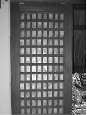
We are given this image of a capiz window:note that it has somewhat of a "fishbowl effect" where the lines are curved around the middle.

Procedure:
**An undistorted portion of the grid is chosen (where the window is parallel to the camera's optical plane), here I've chosen the upper left portion of the window.
**The dimensions of a square in this "ideal" part is measured in pixels (pixel-counting).
** The coordinates of the ideal grid vertex points are then generated, and these were used to compute for c1 to c8 in the following equations:

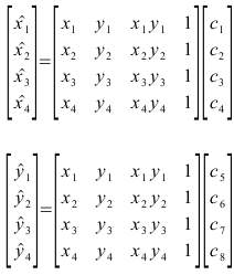
easier to treat in matrix form: and
where: and .

**Now for each pixel in the ideal rectangle, the location of that pixel in the distorted image is calculated for using the following equations:

**If the resulting coordinate is integer-valued, the [greyscale] value is copied from the corresponding pixel of the distorted image onto the blank pixel. Otherwise, the interpolated greyscale value is computed using:

counting the top right capiz shell grid as (0,0), i chose capiz shells (1,3), (2,3), (1,4), (2,4), (1,5) and (2,5) because they seemed the least distorted to me.

the final "fixed" image is shown below:

There's still some distortion, but it is (to me) not as bad as the original image.

i give myself a grade of 9 for this activity. for although the distortion was fixed for the most part, there still some apparent distortion in some parts.

thank you to jeric tugaff and cole fabros.

Activity 11: Camera Calibration

The task: to calibrate our cameras by mapping the real-world 3D coordinates of an object unto its image 2D coordinates.

From the lecture, this mapping is algebraically represented by the following equations where the 2D coordinates (yi,zi) are solved for using the 3D coordinates (x0,y0,z0).

In matrix form, this is written as:
and can be rewritten as: Q = ad
The transformation matrix, a, can then be solved for using:
Activity procedure:

1. take a picture of the provided 3D calibration checkerboard and pick out an origin and 20 edge points.3D calibration checkerboard with chosen points marked with X's
   

Real-world coordinates of chosen points:

x0	y0	z0
8	0	12
4	0	12
0	0	12
0	4	12
0	8	12
4	0	9
0	4	9
8	0	6
4	0	6
0	0	6
0	4	6
0	8	6
4	0	3
0	4	3
8	0	0
4	0	0
0	0	0
0	4	0
0	8	0
0	0	1

2. Use scilab to process the image and use the locate() function to find the image coordinates of the chosen points.
Image coordinates of the chosen points:

yi	zi
17.714286	429.85714
137.71429	411.85714
234.57143	399
324.57143	418.71429
436.85714	443.57143
139.42857	319.28571
323.71429	321.85714
23.714286	219
140.28571	222.42857
237.14286	227.57143
324.57143	224.14286
439.42857	221.57143
142.85714	129
324.57143	130.71429
29.714286	8.1428571
143.71429	35.571429
238	60.428571
326.28571	36.428571
437.71429	6.4285714
238	87

Code:
stacksize(4e7);
im=imread('C:\Documents and Settings\Endura\My Documents\186\DSC04829.jpg');
imshow(im);
x=locate()

3. Use scilab to input the chosen points into the above equation (13), and use the above
equation (15) to solve for the transformation matrix a.
Code:
xo=[8 4 0 0 0 4 0 8 4 0 0 0 4 0 8 4 0 0 0 0];
yo=[0 0 0 4 8 0 4 0 0 0 4 8 0 4 0 0 0 4 8 0];
zo=[12 12 12 12 12 9 9 6 6 6 6 6 3 3 0 0 0 0 0 1];
yi=[18 138 235 325 437 139 324 24 140 237 325 439 143 325 30 144 238 326 438 238];
zi=[430 412 399 419 444 319 322 219 222 228 224 222 129 131 8 36 60 36 6 87];

for i = 1:length(xo)
Q((2*i)-1,:) = [xo(i) yo(i) zo(i) 1 0 0 0 0 -(yi(i)*xo(i)) -(yi(i)*yo(i)) -(yi(i)*zo(i))];
Q(2*i,:) = [0 0 0 0 xo(i) yo(i) zo(i) 1 -(zi(i)*xo(i)) -(zi(i)*yo(i)) -(zi(i)*zo(i))];
d((2*i)-1,:) = yi(i);
d(2*i,:) = zi(i);
end

a = inv(Q'*Q)*Q'*d;

The following values for were obtained:
a =

- 26.918641
12.900713
- 0.7063340
238.39153
- 6.5092147
- 6.8013387
27.705465
59.226318
- 0.0239055
- 0.0275689
- 0.0016180

Testing this calibration using 3 test points, there was a discrepancy of a few pixels. The error average at less than 5% though, and this to me is an acceptable range given that there are many factors that could contribute to the distortion of the image.

i give myself a grade of 10 for this activity. i accomplished the desired calibration with minimal error.

thank you to cole for the help.

Activity 10: Processing Handwritten Text

our mission: pre-processing handwritten text for image-processing.

i chose 3 different parts with writing from the order form image, the three had (or so it seemed to me) varying difficulty for processing.

**code:
stacksize(4e7); im=imread('C:\Documents and Settings\Endura\My Documents\186\act10-1.jpg'); gim=im2gray(im);
fim=fft2(gim);
//fsim=fftshift(fim); //afsim=abs(fsim); //imshow(afsim,[]);xset("colormap",hotcolormap(20)); //outputs fft2 of image (for enhancing)
imf=imread('C:\Documents and Settings\Endura\My Documents\186\act10-1fil.jpg'); //filter
fts=fftshift(imf); ims=fim.*fts; ima=fftshift(ims); //uses filter created to erase in fourier-space horizontal lines from the image
//afsim=abs(ima); //imshow(afsim,[]);xset("colormap",hotcolormap(20)); //outputs fft2 of "cleaned" image
img=abs(fft2(ima)); //imshow(img,[]); //outputs cleaned image
imgb=im2bw(img,0.45); //imshow(imgb,[]);
se=ones(2,2); dil=dilate(imgb,se,[1,1]); ero=erode(dil,se,[1,1]); //closing operator //imshow(ero,[]); //final pre-processed image

[L,n]=bwlabel(ero);

The actual process:

• image is read and converted to grayscale for easier processing
• the fft2 of the original image is processed and displayed to see where the horizontal lines to be deleted are
• a filter is made (GIMP) with black lines that just cover the recurring peaks where the horizontal lines are in fourier-space
• the fft2-ed original image and the fftshift-ed filter are combined to delete the lines and the cleaned output image is displayed, as well as its fft2(to make sure)
  
• the image from the last stage is converted to black and white
  
• the closing operator is used (the opening operator is unnecessary for this activity, and from the trials i had with it, it makes the image worse)
• bwlabel() is used to label the individual letters for handwriting image processing

i ended up using the second image for the activity because the first image had such light-colored letters that it was hard to clean the image without deleting them too, and the third image had too few words in it.

step-by-step outputs:



**i actually tried and re-tried this and avoided posting the report as long as possible even though i finished the activity quite quickly, because i was just never satisfied with the results. Because the words are so small, erasing the lines from the image also erases the middle parts of the letters and using binary operations on it to close that gap only makes the letters run together, so if one wanted this for handwriting-analysis or automated handwriting-reading, it would be useless.

**i give myself a grade of 8 for this activity because i tried my best with it. ]
**thank you to everyone who reassured me that all of theirs were ugly too.

Activity 9: Binary Operations

original image:**Our task: to estimate the cell (punched paper circles) size in pixels.

First, the image is cut up into 9 256x256 images using GIMP to save memory. On the assumption that all the sub-images have the same PDF and CDF, the histogram of one is processed to find the threshold for the next step, and fix the contrast if neccessary.
(The program used is simply that used in activity 4)

Next, in a loop where each sub-image is processed then analyzed individually before returning the final result (thanks to jeric's help with the strcat() function); the following program:
stacksize(4e7);
pre='cir';
counter=1;

for i=1:9
im=imread(strcat([pre,string(i),'.jpg']));
imb=im2bw(im,0.79);
//imshow(imb,[]);

se=[0 1 0; 1 1 1; 0 1 0];
//se=ones(2,2);
dil=dilate(imb,se,[1,1]);
ero=erode(dil,se,[1,1]);
//imshow(ero,[]);

//se1=[0 1 0; 1 1 1; 0 1 0];
se1=ones(3,3);
ero1=erode(ero,se1,[1,1]);
dil1=dilate(ero1,se1,[1,1]);
//imshow(im,[]);

[L,n]=bwlabel(dil1);
for j=1:n
area(counter)=length(find(L==j));
counter=counter+1;
end
end

scf(10);
histplot(length(area),area);
x=find(area<600>400);
scf(11) histplot(length(x), area(x));
a=area(x);
a=sum(a)/length(x) //area
y=stdev(area(x)) //error

i.e. ...first converts the sub-image into binary using the previously determined threshold;
...the CLOSING operator (a morphological operator expressed as a composition of 2 morphological transformations, namely first dilation then erosion using the same structural element, in this case a 3-pixel long, 1-pixel wide cross) is then used to effectively get rid of the "pepper noise" in the image;...after which, the OPENING operator (the dual of the closing operator which is characterized by the use of the tranformation erosion before dilation, using the structural element 2px by 2px square in this case) is used to get rid of the "salt noise" in the image, as well as attempting to separate the nearly-touching "cells" from each other;...the scilab function bwlabel() is then used to label each individual cell, then regions are scanned to obtain the histogram that lays out the measured areas of all the "blobs"/"cells"/circles;**as we can see, the values are spread out a little because of leftover salt noise not totally erased by opening, and the tendency of the program to consider cells that are right next to each other to be just one big blob; to find the actual mean area we get rid of these outliers by only considering those values that range between 400 to 600, an estimate of the parameters wherein the mean area is most likely to be inferred from the above histogram

...this last gives the considered histogram range:and an estimated mean cell area value of 534.51064, with a standard deviation of 22.431415

From the process used, to the obtained histogram and standard deviation value, this is a reasonable estimate. Sources of error are possibly the truncation of a few image details when the image was converted to binary before the opening and closing, and the slight distortion of the circles caused by the choice of structural element/s.


**i give myself a grade of 10 for this activity because the objective was achieved and the obtained final values were quite plausible, not to mention the extra effort benj and i put in initially to enhance the images to separate the stubborn circles. if i actually get that done, i might put that up here as an update.
*thank you to benj,mark leo, jeric

EDIT: for some reason this was saved as a draft while just my initial program from last week was published,i didn't even notice until just now. problem fixed, every picture once again painstakingly uploaded, actual report posted.

Activity 8: Morphological Operations

**I tried to take a picture of my "prediction" paper but with a 2 megapixel phone camera,it's hard to take a decent photograph of anything written, nevermind the total number of pictures that would entail me uploading.

Dilation is defined as a morphological operation where the dilation of A by B denoted by A dilation B is defined as:This involves all z's which are translations of a reflected B that when intersected with A is not the empty set. B is known as a structuring element. The effect of a dilation is to expand or elongate A in the shape of B.

Alternately, Erosion is defined as a morphological operation defined as:The erosion of A by B is the set of all points z such that B translated by z is contained in A. The effect of erosion is to reduce the image by the shape of B.

The activity is to erode and dilate a series of images with a 4x4 square, a 2x4 rectangle, a 4x2 rectangle, and a plus sign with legs 50 pixels long, 1 pixel thick.
using the following scilab code:
im=imread('act8shape.png');
se=ones(4,4);
//replace with (2,4) and (4,2) in turn for the rectangles
//se=[0 0 1 0 0; 0 0 1 0 0; 1 1 1 1 1; 0 0 1 0 0; 0 0 1 0 0];
dil=dilate(im, se, [1,1]);
imshow(dil,2);
ero=erode(im,se,[1,1]);
imshow(ero,2);

**RESULTS:
1)50x50 squareafter dilation:after erosion:
2)triangle with 50 base, 30 heightafter dilation:after erosion:
3)circle with radius 25after dilation:after erosion:
4)60x60 hollow square with border width 4after dilation:after erosion:
5)cross with leg length 50, line width 8after dilation:after erosion:
**i give myself a grade of 10 for this activity, because the scilab results closely matched my predictions.
**thank you to ed for debating with me.